Introduction and Objectives

The German power system is adding renewable energy sources in the north, where wind energy plants reach their highest efficiency, due to higher wind speeds. At the same time old power plants e.g. nuclear, hard coal and lignite are being phased out [^eser-frey_analyzing_2012]. These older power plants were mainly located in southern and central Germany. The energy sink, industrial and private demand, is not shifting north. Therefore, the renewable energy has to be transported from north to south which increases the congestion in the power grid. The amount of offshore wind power, that the German energy system can use, can be greatly increased by adding new power lines ¹.

However, it is not enough to find the shortest route when building new power lines. Other parameters have to be taken into consideration, as the steepness of a road or the soil for example, play an important role for the building cost of a road or pipeline ². When planing the additional routes for a power grid, further aspects such as legal regulations and acceptance by the local population have to kept in mind. Also technical aspects, as the effects on the grid stability are further points to take into consideration ³.

Due to the increasing demand for renewable energy wind offshore wind turbines supplied 5.5 % annual percentage in 2020 of the German energy mix ⁴.

The physical modelling in the power systems models ranges from not modelling the grid at all to models that use of Kirchhoffs laws ⁵. The calculation of a power system is complex, because changing one edge changes the flow in all parts of grid. Besides, the actual grid data are confidential ⁵. Some models not only consider the grid of one nation, but consider neighbouring states or the whole European power system ⁶. Older power grid models are e.g. optimising the well fare, but economic modelling is not sufficient for planning modern routes, as the aspect of environmental sustainability, security of supply and the public acceptance play an increasingly important role ⁷ in modern planning.

In contrast to a GIS analysis, these other factors can be studied done with a [MCDA]{acronym-label=“MCDA” acronym-form=“singular+full”} ⁵. Stakeholders as decision makers can be included and combined with an expert system ⁵.

The uncertainties associated with [MCDA]{acronym-label=“MCDA” acronym-form=“singular+abbrv”} are data uncertainties, preferential uncertainties and model uncertainties are investigated with a sensitivity analysis ⁵ or simulation ⁸. Both inter- and intra-criteria preferential uncertainties ⁹ can be considered.

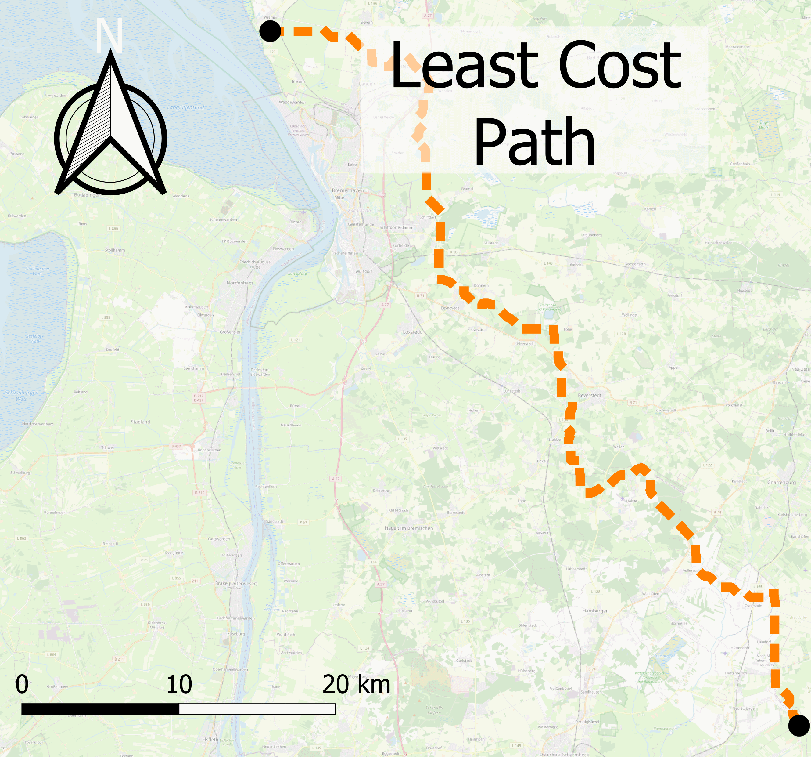
This paper aims to find potential paths for power lines by using the Least Cost Path algorithm. Land usage and planning data are used to estimate the costs arising by using the local area. The task was to provide the Least Cost Path using a [wps]{acronym-label=“wps” acronym-form=“singular+full”}. Beyond that, methods to reduce the needed compute power for finding the Least Cost Path had to be studied.

Methods

The Least Cost Path algorithm is used to plan a potential, cost-optimised route for a power line. The Least Cost Path algorithm is a Dijkstra algorithm ¹⁰ applied on a raster map. The vertices of the graph are the pixel centres, that are connected to the eight neighbouring pixel centres via the edges. This makes it possible to find routes on graphs that are not predefined, such as road networks. The weights of the edges are the local costs of transit from one pixel center to the neighbouring pixel center. The costs can be physical costs, such as the local slope, but also can be composed of other factors as the acceptance rate to transverse a given land usage. The Least Cost Path algorithm consists of at least two successive steps. 1) The first step is to aggregate the costs of travelling from the starting point to a given set of end points. This step generates the aggregated cost raster of travelling from the starting point to any point of the cost raster. 2) In the next step the backtracking, the route of the actual Least Cost Path is calculated. For each end point the path via the lowest cost neighbour is taken until the starting point is reached.

Some implementations switch the roles of start and ending points, so that either many start points and one single end point, or one single end point and many end points can be used. In some implementations there is an extra step between 1) and 2) that calculates cost-weight direction raster, that encodes the direction of the shortest path to the starting point as integer values.

We retrieve a set of different spacial data-sets from public sources as a basis for creating the cost raster. The study area are the counties of Cuxhaven and Osterholz in the state of Lower Saxony, Germany. Areas protected by different European and National conservation laws are provided by the German Environment Agency as [wfs]{acronym-label=“wfs” acronym-form=“singular+full”} ¹¹.

The national land coverage (ATKIS) with a scale of 1:250000 are provided by the Federal Agency for Cartography and Geodesy ¹². The national power grid (tags: ‘power’: line) has been retrieved via OpenStreetMap ¹³. Local data as houses at Level of Detail 1 are provided by the State Office for Geoinformation and Land Surveying of Lower Saxony ¹⁴. In addition, local planning geodata for the land use are taken from ‘Metropolplaner’ (Planning data Lower Saxony & Bremen) ¹⁵.

PyWPS ¹⁶ is used to provide the Least Cost Path algorithm as a [wps]{acronym-label=“wps” acronym-form=“singular+abbrv”} in combination with flask ¹⁷. As client, Birdy ¹⁸ connects to the [wps]{acronym-label=“wps” acronym-form=“singular+abbrv”}, sends the cost raster, starting point, end points and receives the resulting Least Cost Path. The initial implementation of the Least Cost Path algorithm is based on the implementation for the QGIS-Plugin ‘Least Cost Path’ ¹⁹ in version 1.0, but refactored to optionally export the aggregated costs in a command line tool. On top, the [wps]{acronym-label=“wps” acronym-form=“singular+abbrv”} provides the complete Least Cost Path algorithm as a single capability.

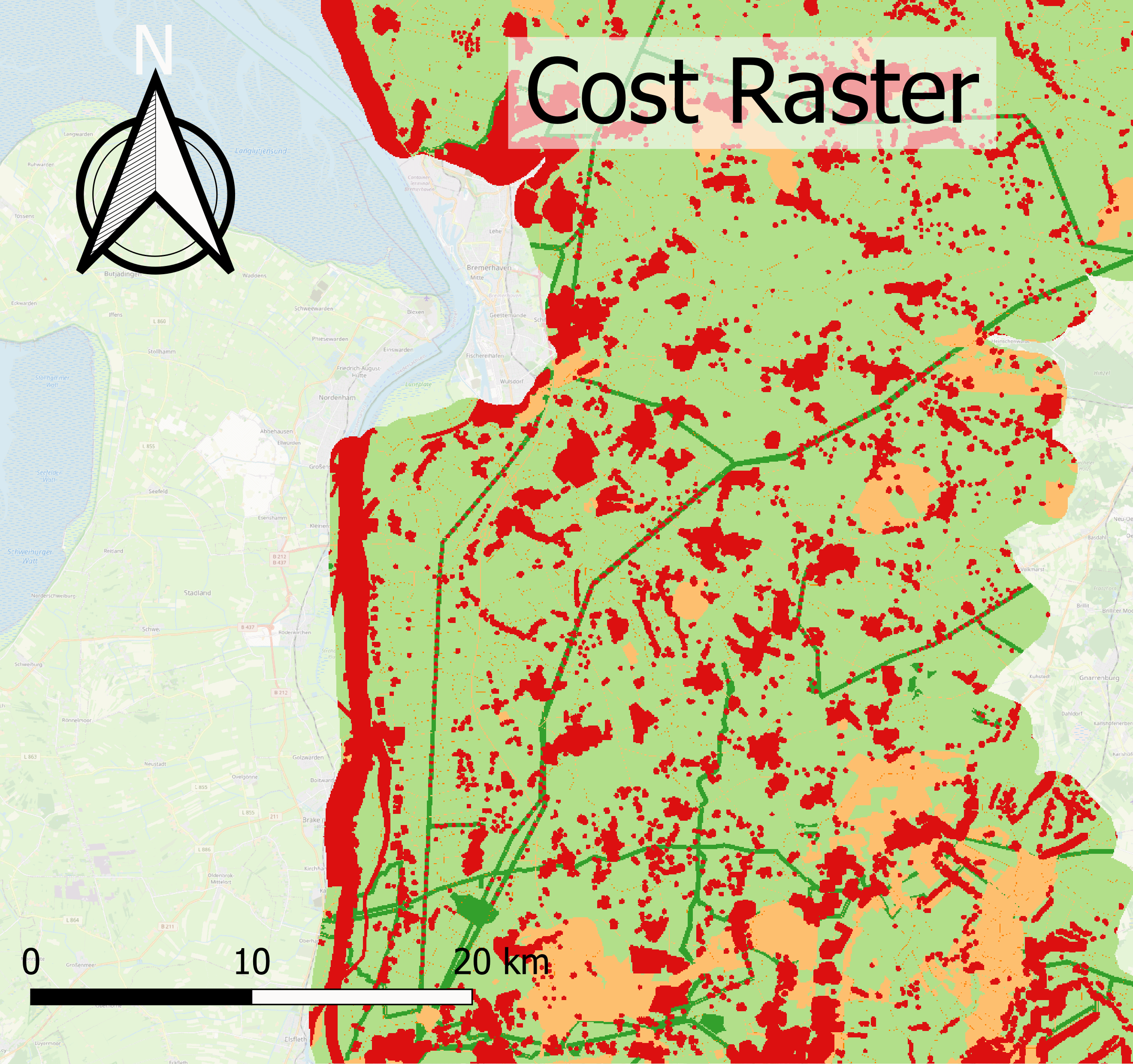
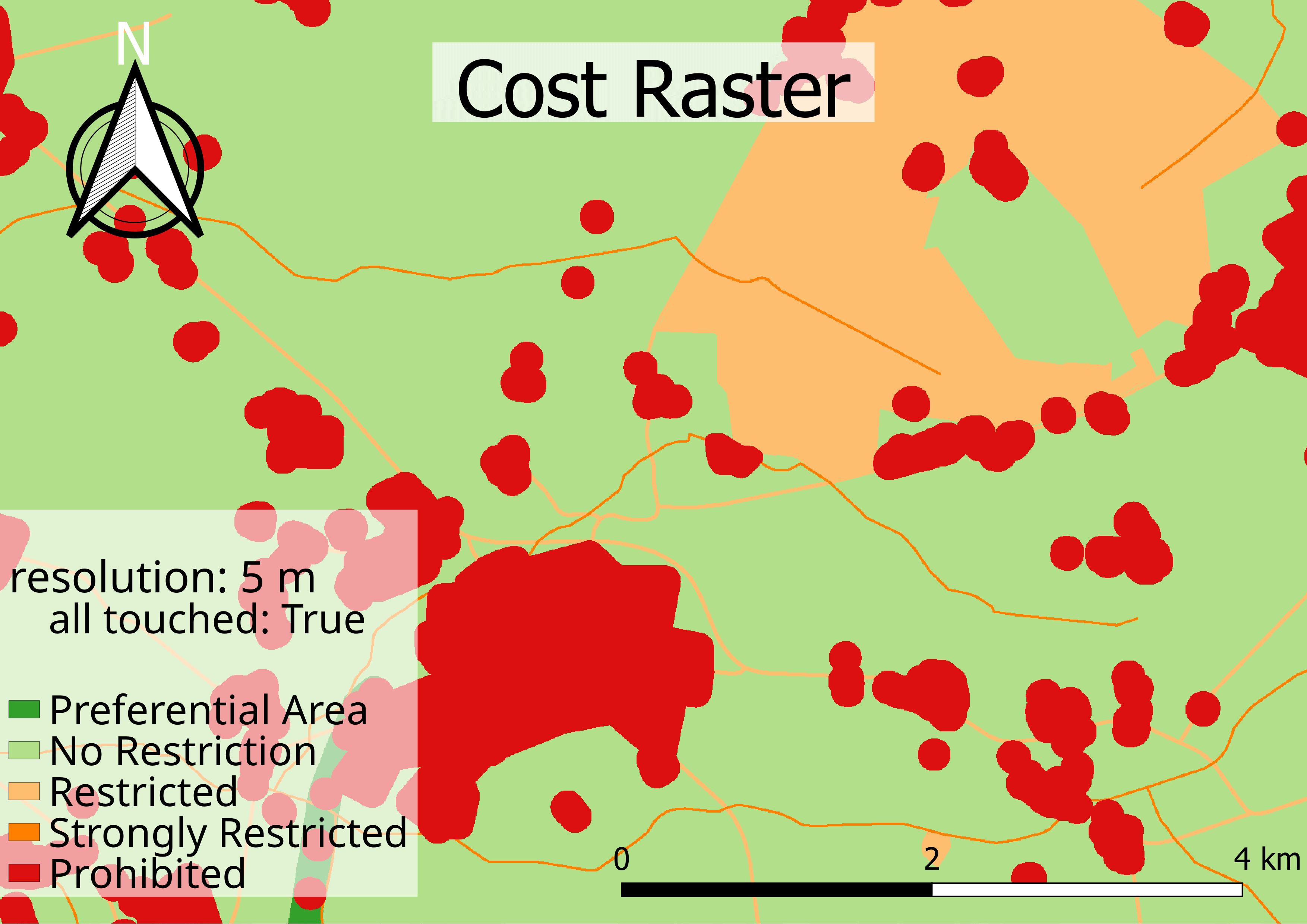
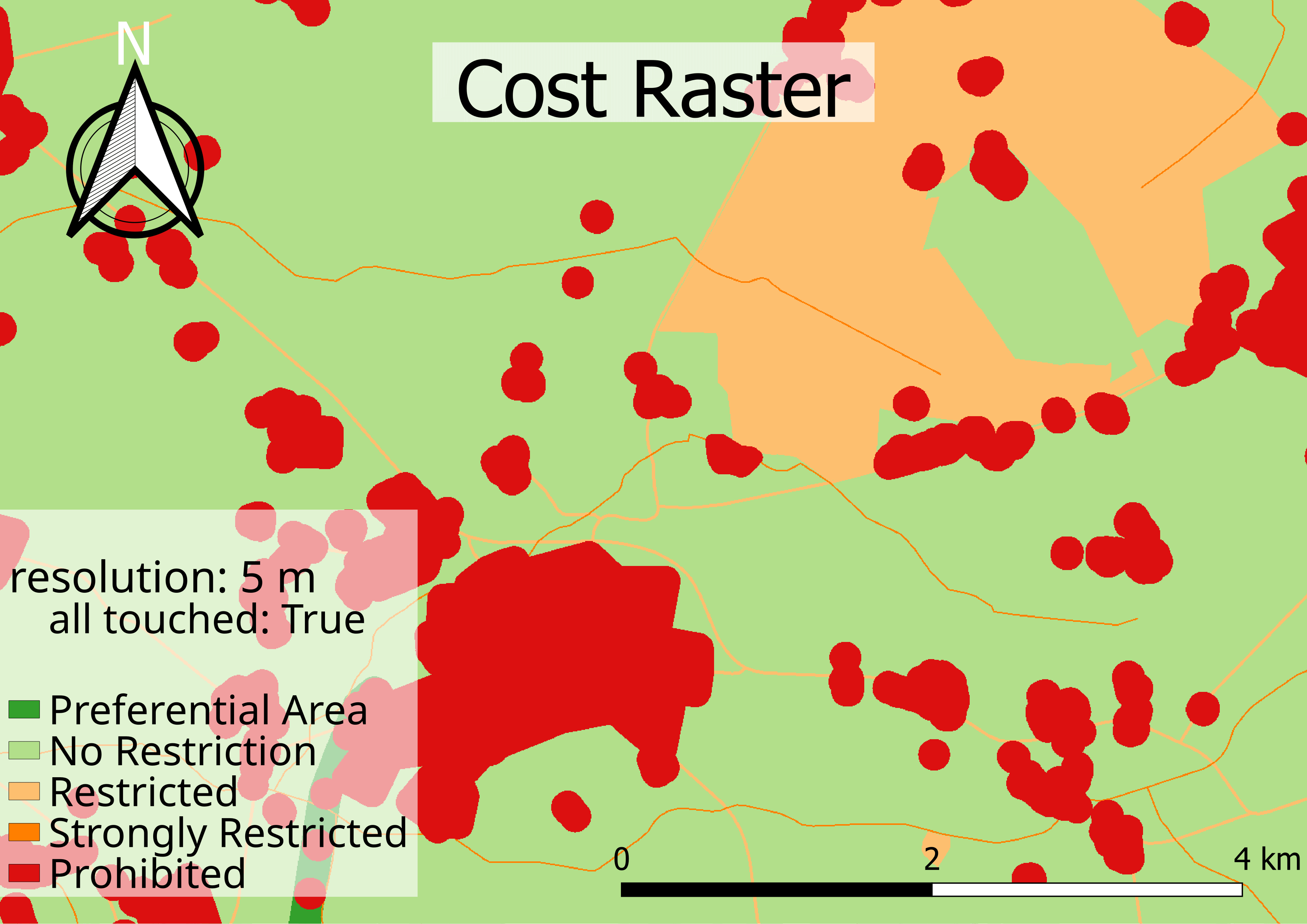
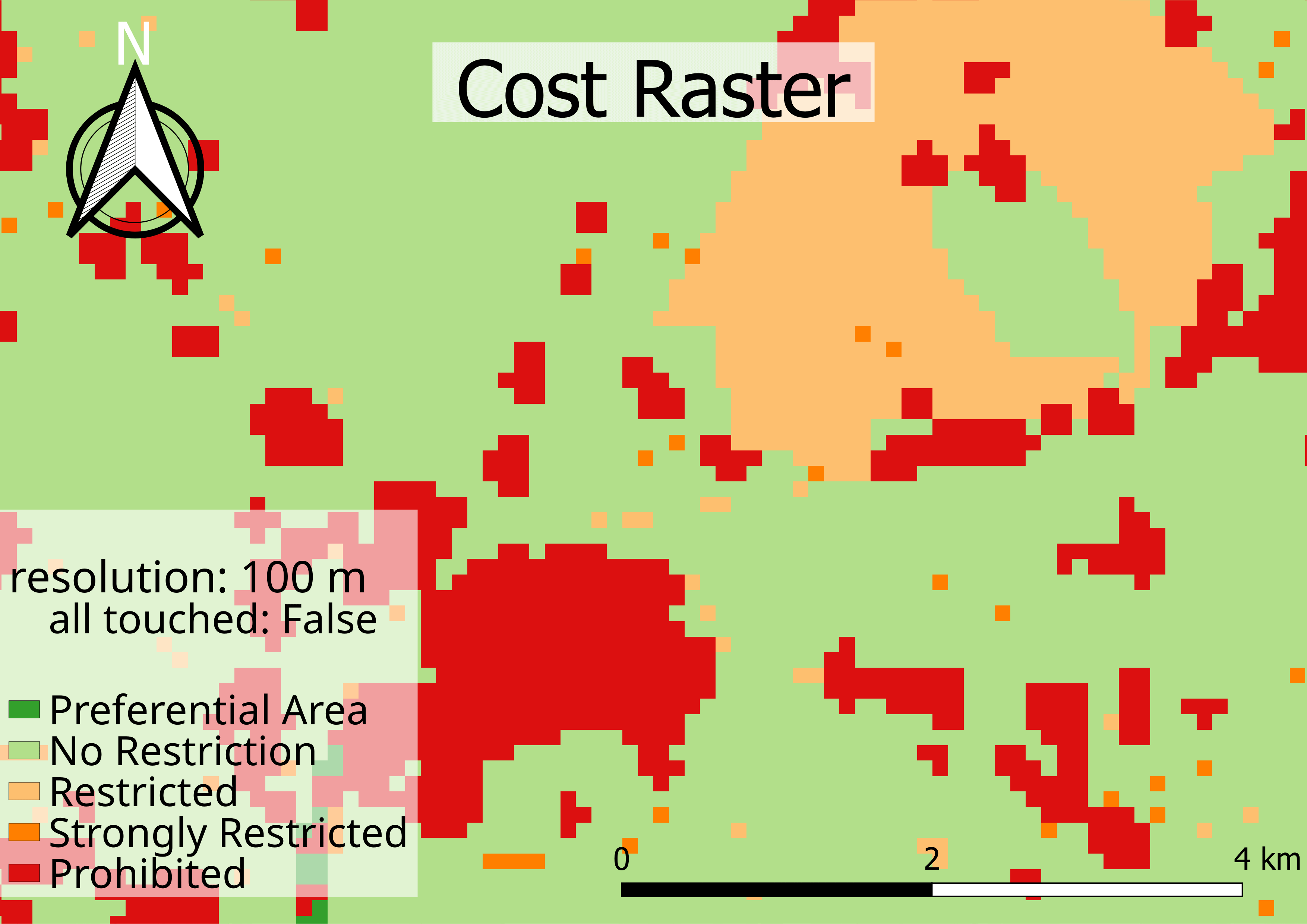
In order to compute intermediate cost raster the different vector layers of the different entities are optionally filtered, buffered and then rasterised. Filtering the layers of the vector files for special attributes enables further differentiation. For example, it is possible to differentiate between heath and uncultivated land in the land cover. Adding a buffer can be used either to convert a line object such as a power line and a road into a polygon (with the correct physical width), or to add minimum distance from an existing of planed area to the new power line. Each of theses intermediate rasters are given a weight (cost) which expresses the cost of using land covered by this layer. In the final cost raster costs of all intermediate rasters are aggregated with the maximum function. Thus, an area covered by several layers is uniformly associated with the highest cost. Any place in the study area, that is not covered by any layer and thus does not yet have a weight, is given the default cost.

The costs have been grouped into five different levels (see table 1{reference-type=“ref” reference=“tab:1”}), starting from Preferential areas with very low costs, via No restrictions, which is the default, used when no other layers are covering the local area, to Restricted, Strongly Restricted and Prohibited areas with high costs. These higher costs represent the degree to which a place with this cost should be avoided, while routing the path. The ratio of the higher costs to the lower costs equals the detour the algorithm is willing to go. Thus, as prohibited areas describe a legal obligation, not to use these areas or only to the utmost minimum, the weight that resembles the costs for these types of areas is set especially high.
All these layers are provided as vectors. The Least Cost Path algorithm uses raster data. Rasterisation transforms a vector into a raster. Rasterisation can be done in two different ways. In both ways, the rasterisation can be imaged, as the old vector is superimposed on the new raster grid with the new given resolution and the new affine transformation and the coordinate reference system of the vector. Both rasterisation techniques differ in the selection of the pixel, that describe the original polygon. A pixels will be selected, if either the centre of that pixel is overlapped by the geo-object, or any part of the pixel is overlaid. Setting all touched to True implies the version with any part of the pixel selected. The version, where an overlapped pixel centre is required, is setting the parameter all touched to False. All touched set to False is considered the default (see figure 1{reference-type=“ref” reference=“fig:alltouched”}).

::: {#tab:1} Cost Level Cost Example

Prohibited 500 National Parks, Buildings
Strongly Restricted 10 Restricted 5 Industrial Areas, motorway, railway
No Restriction 0.5 Default Preferential 0.1 Motorway and Railway Buffers

: Used levels of costs, the applied numerical equivalent and example layer this cost have been used for. :::

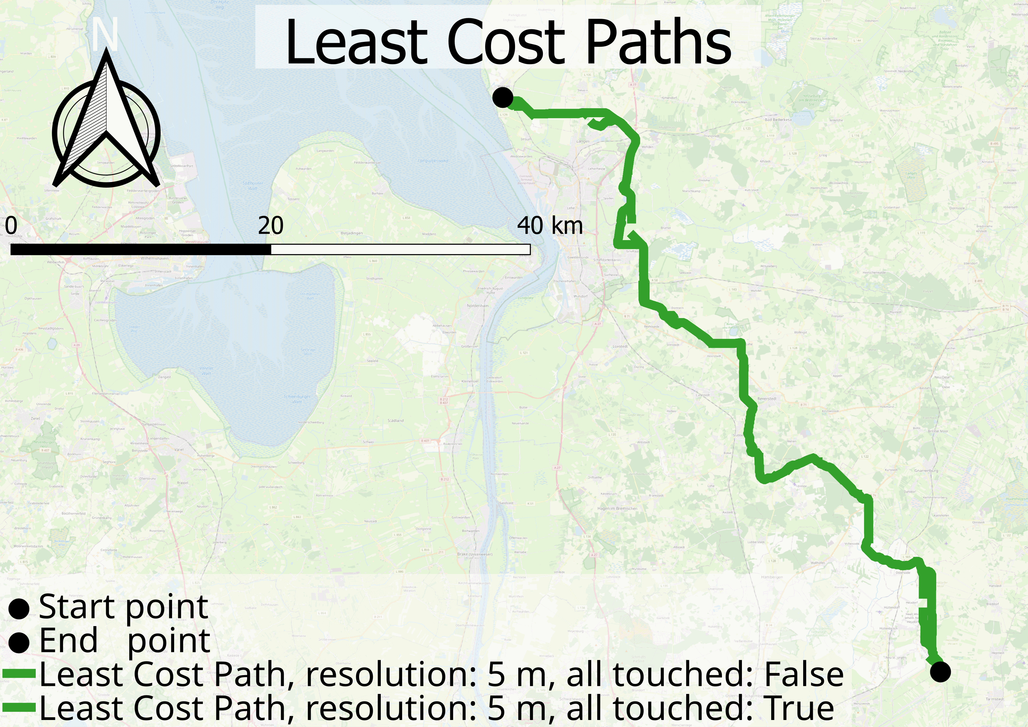
The complete list of layers and the applied processing steps can be found in Supplement S1.

All three steps of the generation of the Least Cost Path: generation of the cost raster, aggregation and backtracking is shown with an example for a cost raster of 50 m resolution and all touched set to False (see 2{reference-type=“ref” reference=“fig:costs2path”}).

The chosen implementation applies early stopping. Therefore, the costs for points that are not needed to try to connect to the end point are not aggregated (see figure [fig:aggregation]{reference-type=“ref” reference=“fig:aggregation”}). After finding an aggregated cost for every end point, the aggregation stops and the backtracking starts. Because the path ends at a power transformer, which is a building type, the paths end at in a Prohibited area. Therefore, areas even further away from the starting point have been explored first.

For low resolution rasterisation, with all touched set to True will show every detail, but the objects are enlarged. When all touched is to False the object only appears, when the is situated at the pixel centre. Thus, this might be used as surrogate, that expresses the likelihood of the object to be sampled and correlates with the object size compared to the pixel size. At high resolution the set all touched to True still overestimates the object size, but the extent is limited. Setting all touched to False will include all objects for high resolution. This setting is most realistic, because the over- and underestimation of the object size is limited to half a pixel size in every direction. The best method should be to use the percentage of the pixel coverage by the object as weight, which is not possible. As an alternative, switching between setting all touched True and False may result in a better assessment of the true costs. When superimposing the resulting cost raster, these map will include both aspects of the correctness: showing every detail and statistically distribute better the real cost. Another method to achieve the same is to downsample high resolution raster.

Results

In this chapter we want to show the different cost rasters, that were created from the same set of layers at different resolutions. The Least Cost Path is estimated from this set of rasters. In the last step the Least Cost Path is computed from the medium resolution rasters and compared with the Least Cost Paths computed from a high resolution raster.

Cost Raster

The cost raster contains all the costs for the geographical region of the study area. The different intermediate cost rasters in the study area are aggregated by the maximum function. If the resolution is higher than the object size, then the effect of setting all touched to True or False is limited. If all touched is set to True and any part of the pixel that is covered by the object, the whole pixel is attributed to the object. This makes the object appear larger. This can be seen in figure 3{reference-type=“ref” reference=“fig:costs_5m”}, which shows a detailed view of the costs for the village of Beverstedt. To set all touched to False is a better description of the real size of the object for high resolution.

In contrast, if the resolution is smaller, all touched set to False leads to a loss of information for smaller objects. Since the default cost is much smaller than the average cost, this method underestimates the cost. The figure 4{reference-type=“ref” reference=“fig:costs_100m”} shows, that for the resolution of 100 m, larger objects are still included in the map, but smaller objects, such as roads, are only partially included.

Least Cost Paths

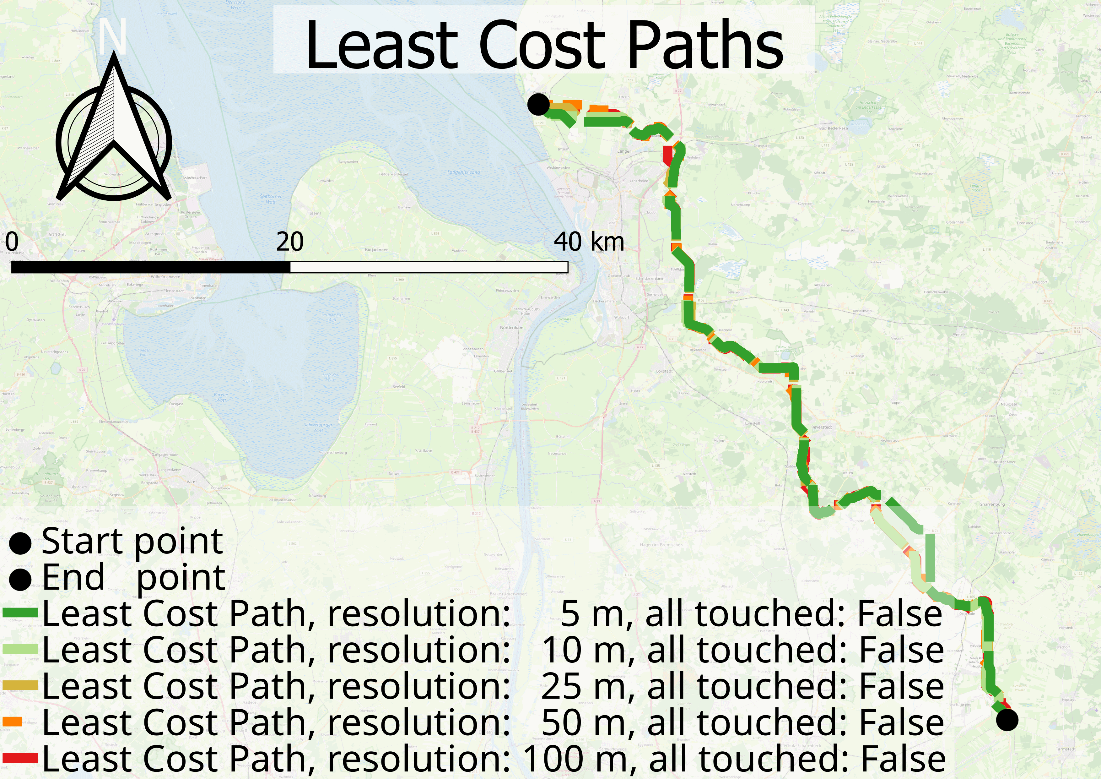
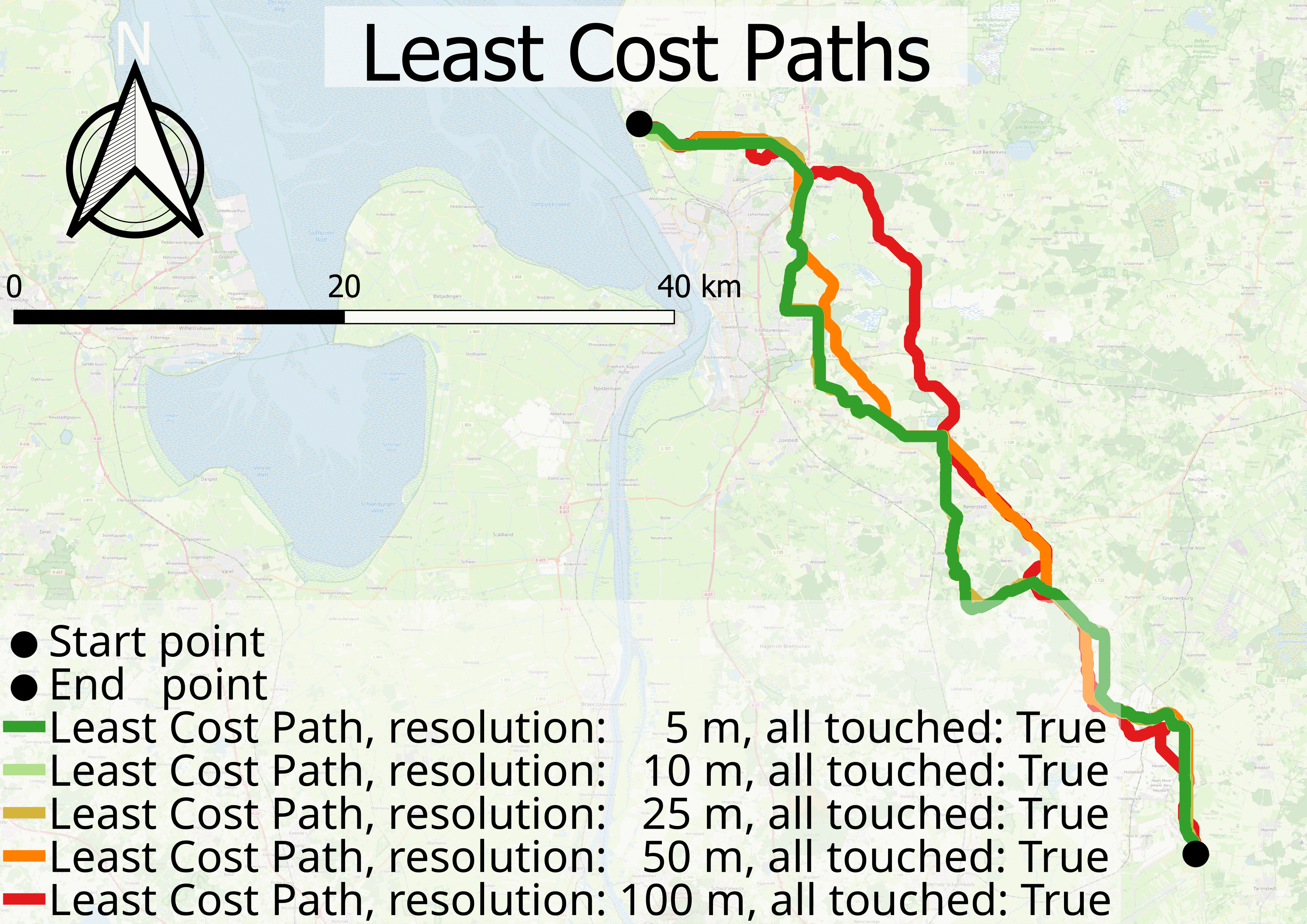
For each resolution the Least Cost Paths were estimated with the all touched set to False and True.

For the study, a starting point was chosen at a transformer about 6 km north of the container terminal Bremerhaven and an end point at a transformer in the southeast of the Osterholz county.

The distance between the paths is calculated by the mean minimum distance. For each vertex $P_i$ in the path $L_1$ the minimum distance between the vertex $P_i$ and the path $L_2$ is calculated and then the minimum distances are averaged (see equation [eq:1]{reference-type=“ref” reference=“eq:1”}). $$\label{eq:1} d_{mean} = \frac{1}{|L_1|} \sum_{i=1}^{n} d_{min}(P_i, L_2) \Bigr\vert P_i \in L_1$$ This equation is used to measure the degree of similarity between the paths. The distances are measured at the same resolution (different setting for all touched), and same setting of all touched (different resolution).

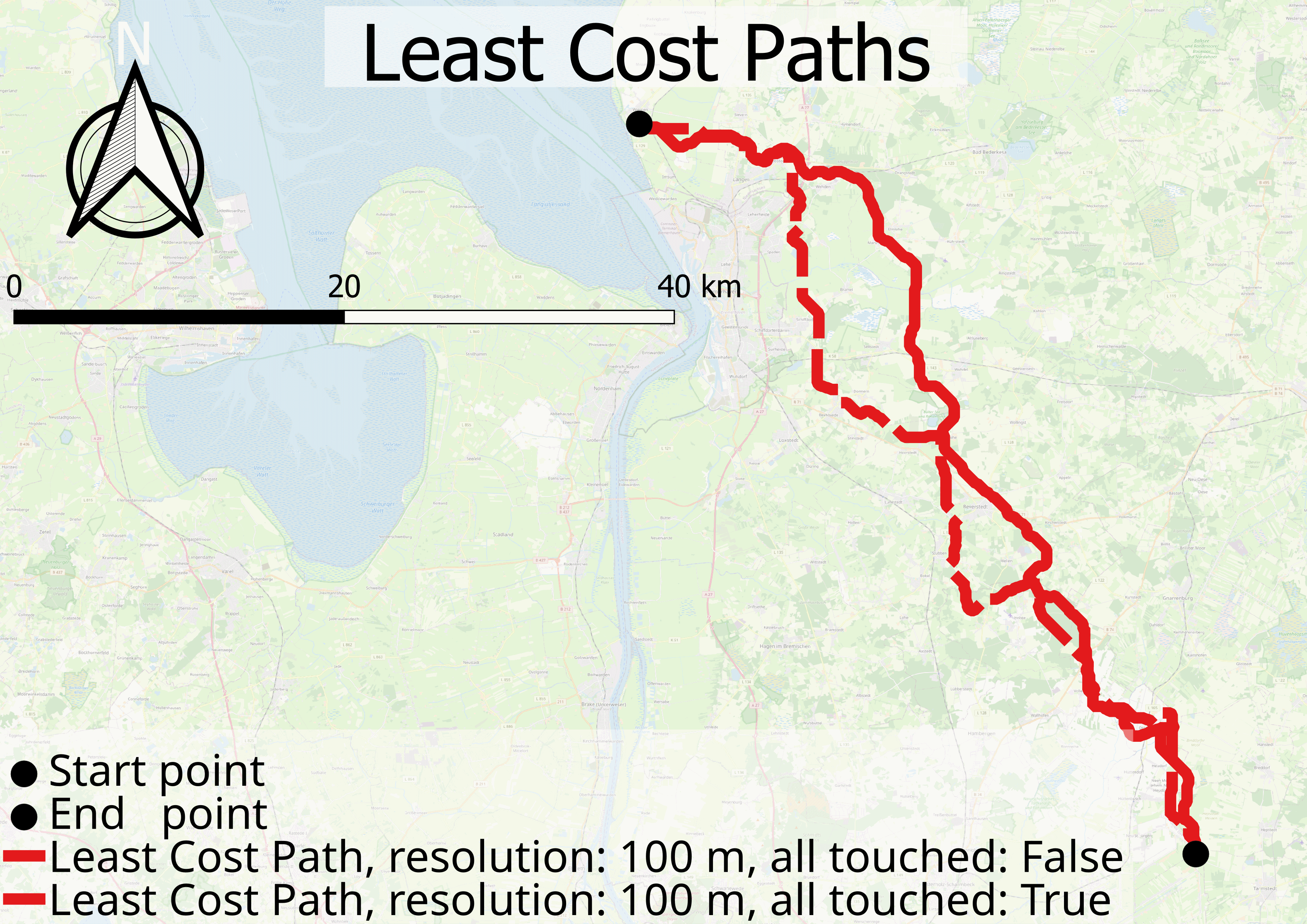
Table [tab:2]{reference-type=“ref” reference=“tab:2”} shows, that the distance between two paths decreases with increasing resolution. In addition, this tendency is depicted in figure 5{reference-type=“ref” reference=“fig:paths_resolution”} for the calculated cost paths of 5 m and 100 m resolutions.

At the same time, the differences in the aggregated costs remain almost constant. Thus the difference between the aggregated costs per resolution decreases. Setting all touched to False underestimates and to True overestimates the costs.

::: table* res /m $l_{al=f} /m$ $l_{al=t} /m$ $d_{mean}$ /m $d_{max}/m$ agg. $cost_{al=f}$ agg. $cost_{al=t}$ $\Delta$ costs agg. $costs_{al=f} \times m$ agg. $costs_{al=t} \times m$

     5         76136.3         78002.0           126.0        1065.0              18665.9              19616.8          -850.00                        93329.6                        97584.8
    10         75430.1         77936.6           277.9        1590.0               8931.2               9731.2          -799.95                        89312.5                        97311.8
    25         75422.9         78422.9           313.8        1621.2               3354.9               3872.7          -517.78                        83871.7                        96816.4
    50         76135.0         70620.0          1140.0        4950.0               1409.0               2300.1          -891.05                        70451.2                       115003.7
   100         76283.8         74120.7          1946.4        6016.6                640.5               1572.3          -931.70                        64051.6                       167226.8

:::

When estimating the distance between the Least Costs Paths from all touched set to True and all touched set to False at the same resolution, the mean minimum distance between the 100 m resolution paths is 1946.41 m and between the 5 m resolution paths is 126.04 m. The similarity between the all touched set to False paths is higher, than for setting to True. The distance for the 100 m path to the 5 m resolution path is 243.42 m for all touched False and 2109.44 m for all touched True.

When cross comparing the similarity between all paths set with all touched set to False and the similarity in between the same resolution, the similarity in between the all touched set to False paths is higher, than for most paths of the same resolution. Namely except for the highest resolution.

This behaviour is shown in figure 6{reference-type=“ref” reference=“fig:paths_alltouched”}. On a more detailed level, it can be seen, that the paths of all touched False also converge directly to the all touched True paths, but the extent is smaller.

The zonal stat (see table [tab:3]{reference-type=“ref” reference=“tab:3”}) for a buffer of 100 m (5 m) around the paths has been used, to estimate the percentage of each costs levels around the paths. When using all touched True at higher resolution the tendency is to use a higher percentage of the Preferential Level and less of the NoRestriction Level. There is no strong tendency for the all touched set to False Least Cost Paths.

:::: table* ::: tabular r r r r r r r r r r r r res /m & all touched & & & & &
& False & 4.7 & (5.4) & 58.7 & (58.9) & 8.8 & (8.4) & 0.7 & (0.7) & 27.1 & (26.7)
10 & False & 19.6 & (33.5) & 68.5 & (64.5) & 1.0 & (0.8) & 0.8 & (0.3) & 10.1 & (0.9)
25 & False & 19.2 & (34.2) & 68.9 & (64.9) & 1.0 & (0.2) & 0.7 & (0.1) & 9.7 & (0.6)
50 & False & 20.4 & (33.2) & 68.0 & (66.2) & 0.9 & (0.1) & 0.7 & (0.0) & 10.1 & (0.5)
100 & False & 21.1 & (30.7) & 69.1 & (68.8) & 1.1 & (0.0) & 0.7 & (0.0) & 7.9 & (0.4)\

5 & True & 18.9 & (28.5) & 67.3 & (66.4) & 1.3 & (1.6) & 1.0 & (0.5) & 11.5 & (3.0)
10 & True & 18.9 & (33.7) & 66.6 & (63.4) & 1.6 & (1.4) & 1.4 & (0.6) & 11.5 & (1.0)
25 & True & 18.7 & (31.9) & 65.5 & (65.5) & 2.0 & (1.3) & 2.5 & (0.7) & 11.4 & (0.6)
50 & True & 9.1 & (13.0) & 75.7 & (83.0) & 3.9 & (2.0) & 4.2 & (1.6) & 7.1 & (0.4)
100 & True & 7.0 & (10.1) & 73.8 & (81.9) & 5.5 & (3.9) & 8.5 & (3.6) & 5.2 & (0.4)
::: ::::

Execution time

In theory, the execution time increases by power of two with the resolution, because higher resolutions result in a higher number of pixels. A double logarithmic fit shows, that the execution time scales with power of $2.1997 \pm 0.007$ of the inverse resolution.

The total execution time consists of two parts: the aggregation of the costs and the back tracking of the least cost to find the path.

Faster Processing of the Cost Path Algorithm

The first step is to optimise the computational speed by a reduced area. Another method is to improve the prediction of the medium resolution itself and thus reduce the need for a computation in higher resolution.

Compare Least Cost Paths from rasters of both all touched settings

For the example paths shown, all touched set to True overestimates ans set to False underestimates the True costs.

A weighted average of the costs could therefore be a more accurate measure and make estimated medium resolution Least Cost Path more similar to high resolution paths. As above example shows the weighting should favour all touched to False.

This will speed-up the aggregation. The time needed for the back tracking stays unchanged.

The optimal ratio of overlaying both all touched for cost raster with 10 m resolution is estimated via similarity of the resulting Least Cost Path to the path of the original high resolution raster. The mean distance of Least Cost Paths from rasters with different ratio is estimated to the path from the all touched set to False raster of the higher (5 m) resolution. Table 2{reference-type=“ref” reference=“tab:4”} shows, that the mean minimum distance decreases with increasing ratio (1:1, 2:1, 4:1) and after this optimum is reached, increases with increasing ratio (8:1, 16:1 and so on). Comparing the similarity of the paths of the different ratios to normal paths with 10 m resolution shows, that paths with a higher ratio of all touched set to True are nearer to the all touched set to True paths. Paths with a ratio in favour of all touched False are much closer to the all touched set to False paths.

::: {#tab:4} r $d_{5~~al=f}$ /m $d_{10~~al=f}$ /m $d_{10~al=t}$ /m

 1:1             119.6              285.5               47.2
 2:1              97.1              263.5               74.2
 4:1              40.1              206.4              100.2
 8:1              41.7              169.0              137.3
16:1              56.7              153.3             152.72
32:1              56.7              145.6              162.1
64:1             163.5               10.6              272.4

: Paths computed from the overlaying of all touched set to False and True raster with the mean minium distance (d) of the paths to the paths calculated from the all touched set to False 5 m resolution and all touched set to False and True raster at 10 m resolution with the ratio (r). :::

Compare Least Cost Paths from downsampled cost raster

As an alternative to the superposition of the rasters of same resolution, a high resolution (5 m) all touched False raster is downsampled to 10 m, 25 m, 50 m and 100 m (bi-linear) interpolation.

The distances from the paths that are computed from the bi-linear downsampled raster to the path of the original 5 m resolution (all touched False) shows, that only downsampling to a resolution of 10 m produces a path that is relatively close the high resolution paths (see table 3{reference-type=“ref” reference=“tab:5”}).

The opposite is true for the lower resolution raster which is more similar to paths computed from the all touched True cost raster. Every path from a downsampled raster is more similar to a path computed from an all touched set to True raster, than to an all touched set to False raster, although the all touched set to False raster of the 5 m resolution was used for downsampling.

::: {#tab:5} res /m l /m $d_{5~m}$ /m $d_{al=f}$ /m $d_{al=t}$ /m

    10   75980.6           59.3           219.4           143.6
    25   70205.3          385.8           558.1           432.8
    50   69217.9          730.8           693.4           255.7
   100   66667.9         1681.3          1605.6           400.6

: Length (l) of the path computed from the bi-linear downsampled raster and the mean minimum distance (d) of the paths from the downsampled raster to the paths calculated from the all touched set to True and False raster of the same resolution as the downsampled raster with resolution (res). :::

Restrict search to a buffer around the Least Cost Paths

Construct a polygon from the two Least Cost Paths (all touched True and all touched False of the same resolution). Buffer the polygon with twice the maximum minimum path distance (see equation [eq:2]{reference-type=“ref” reference=“eq:2”}). $$\label{eq:2} d_{max} = max(\sum_{i=1}^{n} d_{min}(P_i, L_2)) \Bigr\vert P_i \in L_1$$

This strategy results in the same Least Cost Path as with the original high resolution raster.

This reduction of compute power provides the possibility to run a 2.5 m. This clipped 2.5 m raster for all touched set to True changes the path only slightly.

The all touched False raster, on the other hand, leads to a completely new previously unused subroute at the end of the path. Due to the low resolution a small path became passable. This small path is a power line next to a road between protected landscape areas. The road and the protected landscape areas are both restricted areas, while the power line is preferred.

Apply the proposed solutions on other paths

To broaden the view and verify the result, four different routes should be found using the above strategies. Two routes should be found from the starting point to two new points in the south east of the investigated area and two routes should be found from the north and north east of the study area to the end point.

For three of the four routes, the Least Cost Path estimation from the clipped raster was able to calculate exactly the same result. For the fourth path, the Least Cost Path from the 5 m resolution raster was clipped by the buffer around the 50 m resolution paths. The speed up from the clipping of the higher resolution raster depends on the number of pixels that have been clipped.

Bi-linear downsampling the of the high resolution raster to a medium resolution did not result in any benefits compared to an original medium resolution raster. The aggregated cost per resolution of the Least Cost Path from the downsampled raster is higher than the normal medium resolution 10 m raster. In addition, the distance from these paths to the high resolution path is greater than the distance from the original 10 m resolution path to the 5 m resolution path (see table 4{reference-type=“ref” reference=“tab:6”}).

::: {#tab:6} Route Method $length /m$ $costs_{al=f}$ $d_{mean}$ /m

 P1-E       5 m      107889.6         208547.8 
        Clipped      107889.6         208547.8             0.0
           Down       96754.2         212911.0           628.1
           10 m      107232.9         203010.2           103.5
 P2-E       5 m      103706.4         155567.9 
        Clipped      103706.4         155567.9             0.0
           Down       92403.3         158238.6           639.9
           10 m      104249.9         149899.7           177.7
 S-P3       5 m      102187.1          34503.8 
        Clipped       90377.1          37926.1          4465.4
           Down       94125.6          37574.9           742.4
           10 m      102461.6          32446.0            81.2
 S-P4       5 m       96449.2          33865.5 
        Clipped       96449.2          33865.5             0.0
           Down       87861.1          36462.7           796.4
           10 m       96739.5          31899.3            83.5

: Length (l) of the path, the aggregated costs per resolution and the mean minimum distance ($d_{mean}$) to the path created from the 5 m resolution all touched False raster for the four control routes. For the reference path constructed from 5 m and 10 m raster and from 5 m to 10 m downsampled raster and 5 m clipped raster for the routes point1 to end point (P1-E), point2 to end point (P2-E), starting point to point3 (S-P3) and starting point to point4 (S-P4). :::

Discussion

In theory, the need for computing time increases with the resolution as power of two. Similarly, the use of main memory increases. This again limits the number of data points, that can be processed and the resolution, and probably causes difference in increase of computation time from power of 2 to a power of 2.2, because additional slower ram moduls has been used for the aggregation of higher resolution.

On the other hand, the similarity to higher resolutions only scales linear with the resolution. Thus, there is a diminishing return of smaller errors, compared to compute time and resources used.

Therefore, this work attempts a) to reduce the computation power needed and b) reduce the deviation for a given resolution compared to a higher resolution raster.

For a), to reduce the computational complexity, clipping of the high resolution has been applied, to reduce the search space of the aggregation. While this method reduces the computation time and memory usage, the backtracking part stays unchanged.

For b), two methods have been used to increase the similarity of the paths computed from the medium resolution raster, to the paths of the highest resolution raster. These methods are used as surrogates for the more complex calculation of the Least Cost Path with the higher resolution. In the first method a bi-linear downsampling of the higher resolution raster has been applied and in the second method, the all touched set to False and True rasters were averaged in different ratios, to compute the optimum weighted cost raster. While the second method of using an averaged raster, shows a higher similarity to the path from the highest resolution raster, the downsampling method is simpler and does not need to be optimised for the given cost. This disadvantage could be reduced by normalising the costs. The fact that downsampling leads to paths that are closer to all touched True, can be attributed to the fact, that all objects are included, such as in to all touched True.

This shows that the way the cost raster is created in the first place can play a crucial role in the end result. So, a nuance can cause a detour. When this behaviour occurs, the polygon may not include the Least Cost Path. This polygon should therefore be overlapped with a polygon around the shortest path. For the set of control paths downsampling could not outperform the original medium resolution rasters.

Early stopping may result in suboptimal paths around the end points for some edge cases, where the connection via another neighbour might be more optimal.

The set of rules, that are used to create the intermediate cost raster, includes a rule to create buffer around buildings which is set to the level Prohibited areas. In all touched set to False rasters the resolution of the medium level raster needs to be high enough to show every detail, at least in the magnitude of the minimum object size plus twice its buffer. This is true for the 10 m resolution raster and less true for the 25 m resolution raster, that misses some details for roads for all touched False raster. Other details such as rivers and houses are already included in the lower resolution raster, due to larger buffers. The raster with all touched set to False might miss some objects, but the missing chance is propotional to the object size and the extent of overestimation is reduced. The Least Cost Path algorithm searches for an optimal path as a line. As lines do not have a width, the route found might contain bottlenecks, that have a smaller width than the object that should be placed there. Therefore, the used resolution should not be smaller than the width of the object that should be placed. This can not be avoided by downsampling, but by weighting the medium resolution all touched True and False rasters.

This paper examines the effect of computational costs and deviation of the results for a limited set of points. Also, only the cost of finding the Least Cost Path from a single starting point to a single end point has been considered. If multiple endpoints are used, the computational cost for the aggregated cost raster has to be paid only once.

If multiple paths are calculated from a single raster, the speed-up benefit is reduced. Especially pre-calculation on medium resolution raster and clipping around a buffering of the resulting medium resolution paths becomes less effective, because as the number of paths increases, fewer pixels are clipped. The Least Cost Path algorithm does only select the single most cost-effective path. Therefore, paths of similar, but slightly higher costs remain unknown. In additional, slight variations on the costs rasters can lead to very different paths, although the costs will not change much. End-users may be interested in selecting a path from a set of similar aggregated costs and applying their own evaluation criteria. This can be achieved a by adjusting the backtracking and return polygons, or by applying perturbation on the costs.

In this work, the intermediate cost layers are aggregated by the maximum function. Other possible aggregation functions are the sum and average functions. Each aggregation function can be justified by a different interpretation of the cost and its scale.

When the Prohibited level is used as the highest level, then summing the two highest levels would result in a new highest level. Also, the maximum function does not interfere with the nodata value. This can be done by a nansum- / nanmean-function, if the nodata value is set to not a number during the aggregation. The disadvantage of aggregation with the maximum function is, that this aggregation is unable to distinguish between nuances of different overlapping intermediate costs. On sum or average aggregated rasters, one can distinguish between different sublevels.

All touched False rasters produce more similar results than all touched True raster, which is probably due to the fact, that the default level is relatively low. As the default level increases, the effect would probably be reduced for low resolution rasters. For high resolution raster, the effect would still be present, because the use of the pixel centre for sampling, reflects the original geometry better.

This effect of the similar aggregated costs per resolution could also be seen in the test paths, even when the paths varied greatly. This could be an indication of an even spatial distribution of the costs.

The all touched set to True cost raster shows every detail, but the sampling with all touched set to True increases the size of the features. The fact that the aggregated costs per resolution for all touched True rasters overestimate the costs when computing the path from a low resolution raster, might be due to the fact, that the high costs are much more frequent, as they are exponential scaled.

Conclusion

The computing costs of the Least Cost Path scales with the square of the resolution. The difference between the aggregated costs of the paths per resolution computed from the all touched set to False raster and the all touched set to True raster only shows a linear decrease. Therefore, the gain in accuracy per compute time decreases. The presented methods attempt to circumvent this bottleneck. When these strategies are applied to a medium resolution raster, the compute time for high resolution results can successfully be reduced without compromising the run time for worse distances to the Least Cost Path from the high resolution raster. The paths can change significantly even for a small change in total cost. Therefore, developing an alternative backtracking algorithm, that generates a corridor of costs might be a good strategy to offer alternative paths and at the same time show variations between these paths. An alternative would be to specify a range of costs and compute the aggregation of the costs and than superimpose these aggregations and compute the path by backtracking from the superimposed cost raster. This again increases the computation time.

In an actual search for the Least Cost Path of a power, a survey could be used as a method to estimate the costs. If the sample size of the survey is large enough, the weights could take into account local differences in relative acceptance.

Only changes in the algorithm have been applied in the search for acceleration. Therefore, other methods such as just-in-time compilation have not been tested.

References

Leuthold, Florian U. ; Rumiantseva, Ina ; Weigt, Hannes ; JesKe, Till ;HiRschhausen, Christian von: Nodal Pricing in the German Electricity Sector -A Welfare Economics Analysis, with Particular Reference to Implementing Off-shore Wind Capacities. In: SSRN Electronic Journal (2005). http://dx.doi.org/10.2139/ssrn.1137382. – DOI 10.2139/ssrn.1137382. – ISSN 1556–5068 ↩︎
Suleiman, Sani ; AgaRwal, V C. ; Lal, Deepak ; Sunusi, Aminuddeen: Optimal Route Location by Least Cost Path (LCP) Analysis using (GIS), A Case Study. In: International Journal of Scientific Engineering and Technology Research 4 (2015), Oktober, Nr. 44, S. 9621–9626 ↩︎
SchÄfeR, Benjamin ; Pesch, Thiemo ; ManiK, Debsankha ; Gollenstede, Julian; Lin, Guosong ; BecK, Hans-Peter ; Witthaut, Dirk ; Timme, Marc: Understanding Braess’ Paradox in power grids. In: Nature Communications 13 (2022), September, Nr. 1, 5396. http://dx.doi.org/10.1038/s41467-022-32917-6. – DOI10.1038/s41467–022–32917–6. – ISSN 2041–1723. – Number: 1 Publisher: NaturePublishing Group ↩︎
Nettostromerzeugung in Deutschland 2020: erneuerbare Energien erstmals über 50 Prozent - Fraunhofer ISE. https://www.ise.fraunhofer.de/de/presse-und-medien/news/2020/nettostromerzeugung-in-deutschland-2021-erneuerbare-energien-erstmals-ueber-50-prozent.html. Version: Januar 2021 ↩︎
BeRtsch, Valentin ; FichtneR, Wolf: A participatory multi-criteria approach for power generation and transmission planning. In: Annals of Operations Research 245 (2016), Oktober, S. 177–207. http://dx.doi.org/10.1007/s10479-015-1791-y. – DOI 10.1007/s10479–015–1791–y ↩︎ ↩︎ ↩︎ ↩︎ ↩︎
DietRich, Kristin ; Leuthold, Florian ; Weigt, Hannes: Will the Market Get it Right? The Placing of New Power Plants in Germany. In: Zeitschrift für Energiewirtschaft 34 (2010), Dezember, Nr. 4, 255–265. http://dx.doi.org/10.1007/s12398-010-0026-9. – DOI 10.1007/s12398–010–0026–9. – ISSN 1866–2765 ↩︎
Hauff, Jochen ; HeideR, Conrad ; ARms, Hanjo ; GeRbeR, Jochen ; Schilling, Martin: Gesellschaftliche Akzeptanz als Säule der energiepolitischen Zielsetzung. In: ET, Energiewirtschaftliche Tagesfragen 61 (2011), Oktober, Nr. 10, 85–87. https://www.osti.gov/etdeweb/biblio/21522981 ↩︎
ButleR, John ; Jia, Jianmin ; DyeR, James: Simulation techniques for the sensitivity analysis of multi-criteria decision models. In: European Journal of Operational Research 103 (1997), Dezember, Nr. 3, 531–546. http://dx.doi.org/10.1016/S0377-2217(96)00307-4. – DOI 10.1016/S0377–2217(96)00307–4. – ISSN 0377–2217 ↩︎
BeRtsch, Valentin ; TReitz, Martin ; GeldeRmann, Jutta ; Rentz, Otto: Sensitivity analyses in multi-attribute decision support for off-site nuclear emergency and recovery management. In: International Journal of Energy Sector Management 1 (2007), Mai, Nr. 4, S. 342–365. http://dx.doi.org/10.1108/17506220710836075. – DOI 10.1108/17506220710836075 ↩︎
DijKstRa, E. W.: A note on two problems in connexion with graphs. In: Numerische Mathematik 1 (1959), Dezember, Nr. 1, 269–271. http://dx.doi.org/10.1007/BF01386390. – DOI 10.1007/BF01386390. – ISSN 0945–3245 ↩︎
Schutzgebiete in Deutschland. https://geodienste.bfn.de/schutzgebiete?lang=de. Version: 2015 ↩︎
Digitales Landschaftsmodell 1:250 000 (Ebenen). https://gdz.bkg.bund.de/index.php/default/open-data/digitales-landschaftsmodell-1-250-000-ebenen-dlm250-ebenen.html. Version: 2021 ↩︎
Boeing, Geoff: OSMnx: New methods for acquiring, constructing, analyzing, and visualizing complex street networks. In: Computers, Environment and Urban Systems 65 (2017), September, 126–139. http://dx.doi.org/10.1016/j.compenvurbsys.2017.05.004. – DOI 10.1016/j.compenvurbsys.2017.05.004. – ISSN 0198–9715 ↩︎
OpenGeoData.NI. https://opengeodata.lgln.niedersachsen.de/#lod1. Version: 2022 ↩︎
Metropolplaner. https://metropolplaner.de/metropolplaner/. Version: 2022 ↩︎
Welcome to the PyWPS 4.3.dev0 documentation! — PyWPS 4.3.dev0 documentation. https://pywps.readthedocs.io/en/latest/index.html. Version: 2016 ↩︎
Flask. https://palletsprojects.com/p/flask/ [^eser-frey_analyzing_2012] EßeR-FRey, Anke: Analyzing the regional long-term development of the German power system using a nodal pricing approach. http://dx.doi.org/10.5445/IR/1000028367. Version: 2012 ↩︎
Birdy — Birdy 0.8.1 documentation. https://birdy.readthedocs.io/en/latest/ ↩︎
LeastCostPath/dijkstra_algorithm.py at master · Gooong/LeastCostPath. https://github.com/Gooong/LeastCostPath. Version: Dezember 2022 ↩︎

Last modified on 2023-03-15